Landing AI in Game Production · Form 2 «Read the Board, Discern the Formation»: Game-Scene Understanding Through Image Masks and Semantic Abstraction
Series intro: “The Kung-Fu Manual for Landing AI in Game Production” records the road I took—every step of it paid for in blood and tears.
In Form 1, «Within Easy Reach», we taught AI to recognize every asset in a project. It knows which Jiangnan-style low shrubshrub_jn_01arefers to. But that is not enough: recognizing every piece on the board does not mean understanding the formation. In Form 2, «Read the Board, Discern the Formation», we teach AI to understand the “formation” an artist has arranged across a map.Note: almost every article in this series is handcrafted. If you only care about the result and not the implementation, feel free to skip Chapters 3 through 6.
1. Origin: A Scene AI Cannot Understand
In Form 1, semantic encoding taught the AI to recognize individual assets. This time, the question is: where am I?
As everyone knows, an LLM does not understand a scene. Even if you hand it a screenshot, it still cannot read the elaborate formation an artist has built:
① "What kind of visual style does this area have?"
     → AI: Make up something plausible.
② "Find the treasure chest beside a staircase."
     → AI: Traverse the World Outliner and inspect objects one by one. Which one is beside a staircase? No idea.
③ "Here is a screenshot. Where is this location in my open world?"
     → AI: What on earth am I looking at?
④ "Find a cave I built out of piled rocks."
     → AI: @#¥%……&*
Those are the problems this article sets out to solve. Map understanding turned out to contain too much material for one article, so I am splitting it into two: this one is about understanding the map, while the next will cover vector search across the entire map.
After this round of training, your AI will be able to understand a map in the real sense of the word, much as a person does, and memorize every scene and position it has sampled. For viewpoints that were never captured, I plan to infer them by interpolating between neighboring views, ultimately enabling millisecond-level lookup at any position in a large open world.
2. What Does It Mean to Understand a Scene?
Consider what happens when a person sees a scene.
First, they see the game world: “Huh, it is pitch-dark in here.” (visual)
Then they sense the spatial relationships: “Wait, there is some light ahead.” (spatial)
Finally, they understand what the scene means: “Oh—this must be the White Bone Demon’s cave.” (semantic)
How would they describe the scene to someone else?
I just found a place. You enter it by pressing E near Black Well. It is even darker than the cave at Flower-Fruit Mountain. I think it must be the hidden boss White Bone Demon’s lair.
From that description, I separate understanding from expression:
| Perception \ Expression | Reference | Comparison | Metaphor |
|---|---|---|---|
| Visual information | 🟢 Identify by visual style | 🟡 Compare density and style intensity | 🟠 Use cultural imagery to describe texture or style |
| Spatial information | 🟡 Identify by spatial position | 🟡 Compare relative position and distribution | 🟠 Describe spatial form through another object |
| Semantic information | 🟡 Identify by function or use | 🟠 Express preference or negation | 🔴 Describe function and narrative through metaphor |
Difficulty: 🟢 easy | 🟡 medium | 🟠 hard | 🔴 extremely hard. The harder cells are difficult for AI both to understand and to express accurately.
The vertical axis—the perception layer—corresponds to three abilities an AI needs in order to understand a scene:
- Visual information — What does this area look like? Style, density, texture, and aesthetic impression.
- Spatial information — How are A and B arranged in space? Who contains whom, what touches or intersects what, what supports what, and what occludes what: topology + direction + distance + support + occlusion.
Topological relations—RCC-8’s DC / EC / PO / EQ / TPP / NTPP and so on—are already a mature area of qualitative spatial reasoning; see Cohn and Renz’s classic survey, Qualitative Spatial Representation and Reasoning. Support and occlusion are often treated separately in vision research, as in Biederman’s 1982 discussion of Support / Interposition. In an engine, however, they ultimately come from the same geometric data, so this framework groups them together by data source. - Semantic information — What is A doing here, and what narrative role does it serve?
- Object meaning — What does this individual object imply?
- Compositional meaning — What does a group of objects mean together? This is mereology: for example, a gap hollowed out from a pile of rocks becomes a cave.
- Design semantics — This scene is run-down because it is meant to depict a village suffering through famine.
- Co-occurrence — Do A and B often appear together? Which pairings are stable?
This level touches several different fields at once: distributional semantics, RDF for knowledge representation, and FrameNet for frame semantics. Co-occurrence is learned from frequency or vectors, not calculated from geometry. Modeling how the current state affects the next state would move further into Markov models. I treat co-occurrence as part of semantics because it expresses scene logic above the level of individual geometry. That topic is somewhat beyond the scope of this article.
The horizontal axis—the expression layer, meaning whether the system can restate what it has learned, covers three strategies:
- Reference corresponds to deixis: shared attention anchors both parties to the same object even without coordinates.
- Comparison uses vague quantifiers and vague language. It need not produce an exact number; it can instead communicate direction, degree, and an implied baseline.
- Metaphor corresponds to conceptual metaphor or cross-domain mapping: shared cultural experience is used to express space, texture, or function that would otherwise be difficult to state directly.
An ideal AI scene-understanding tool should, in theory, cover every cell in that 3 × 3 matrix.
A good agent also needs a long-term scene memory: if we discussed something before, it should be able to retrieve it when the subject comes up again.
Now let us talk about implementation.
3. Stop Talking Only About MCP: It Is a Bottomless Pit
What we actually need is a translation layer between engine data and the LLM: something that extracts whatever the LLM wants to know from the engine, then translates it into a form the model can use. MCP is the obvious first thought.
MCP has indeed been extremely popular for a while.
But MCP is not a pleasant job if what you want is a fast, dramatic payoff. It demands a great deal of engineering and tuning. Over the past few months I have spent an enormous amount of effort debugging it, even developing a tuning methodology and staring at telemetry every day. Honestly, the result is still not as good as I want.

Why?
If you have used any UE MCP tools, you have probably encountered several problems in the scene-understanding layer:
It cannot truly understand the style I am asking about.
A person can look at a field and describe whether the grass is sparse or dense. The tool cannot “understand” or summarize that impression.Context explodes as the tool count grows geometrically.
Many MCP implementations expose interfaces originally designed for UI directly to the LLM. That is like handing a swordsman a kitchen knife: usable, but awkward. UI was designed for people; its architecture never accounted for limited context windows, hallucination, and the other weaknesses of an AI.More tasks mean more interfaces.
An atomic tool signature is fixed. Afindtool may begin as a name search, but the requests quickly become “find a treasure chest beside a staircase” (neighborhood reasoning), “find a shrub in this visual style” (semantic filtering), or “count the rocks in this area” (aggregation). The samefindnow hides several fundamentally different computations. One rigid interface cannot span all of them: either the number of tools explodes or the depth of analysis collapses. My testing also found that offering more MCP tools can actually lower completion rate—not because the tools lack capability, but because the model no longer knows which one to choose.There is no validation, so one bad step poisons everything after it.
Every tool call can fail. Most MCP systems only “provide data”; they do not tell you whether the data is correct. If the agent says there is a pine tree atxxx, should you believe it? Without a mirror in which it can inspect its own work, errors snowball through multi-step reasoning until the whole task drifts off course.It is slow and expensive—often slower than doing the job yourself.
Every probe crosses a bridge, waits for the editor, and burns tokens. By the time it finishes a lap, I could have clicked through the task myself. A system whose nominal capabilities cannot beat the time and cost of a human using the editor directly has no place in serious production.
MCP is not the only option available to us:
| Approach | One-line principle | Per-call latency | Context | Read/write | AI compatibility | Cross-version | Compute per call | Fatal flaw |
|---|---|---|---|---|---|---|---|---|
| MCP | Run an MCP server in the engine via JSON-RPC | 🟡 seconds | 🔴 every interface exposed | ✅ | 🟢 protocol-native | 🔴 tied to APIs | 🟡 | slow + expensive + context explosion + wrong granularity |
| CLI + Commandlet | Launch headless UE to run a command | 🔴 30s+ startup tax | 🟢 persisted output | ✅ | 🟡 needs another parser | 🟡 tied to versions | 🔴 process fork | cold start makes interaction impossible |
| Exported text snapshot | Cook the scene into JSON/XML on disk | 🟡 seconds | 🔴 explodes on large scenes | 🔴 read-heavy | 🟡 superficially friendly | 🟡 brittle format | 🟡 | stale + one-way + brittle |
| OpenUSD | Standardized scene description with bidirectional I/O | 🟢 seconds | 🟡 structured | ✅ | 🟢 text-native | 🟢 stable standard | 🟢 | not unified across the game industry |
| Direct screenshots | Render + let a VLM inspect the image | 🔴 tens of seconds | 🔴 image tokens | 🔴 observation-heavy | 🟢 multimodal-native | 🟢 flexible | 🔴 very high | expensive + view/render-state dependent + loses structure |
By where the information comes from, those five approaches form three groups:
MCP + CLI acquire information online through engine interfaces. The data is fresh and reflects the current scene, but the interfaces must be maintained, the returned payload can be huge, and every engine upgrade carries a migration cost.
Exported snapshots + OpenUSD reconstruct the scene from offline data. They avoid occupying a running editor, can be versioned, and are convenient for cross-tool workflows, but they are stale and large scenes can produce enormous snapshots.
Direct screenshots acquire information through images + a VLM, much closer to how a person observes a scene. Their semantic intuition is strong and they are flexible across engine versions, but the ceiling is set entirely by the VLM’s visual ability and by the information present in the image.
Only children choose one. I want all of them—combined in pairs.
For the three kinds of information on the vertical axis of the earlier 3 × 3 matrix, I propose three corresponding implementations:
- Visual information ➡️ 2D asset masks: VLM screenshots + exported snapshot text, extending what an image can communicate.
- Spatial information ➡️ GSDL, the General Scene Description Language: a variable-granularity, human-language-level USD + MCP layer that tackles context explosion and weak spatial perception.
- Semantic information ➡️ Vector Atlas, map-wide semantic encoding: Commandlets combined with the two methods above. The implementation has enough difficult bottlenecks to deserve a separate article.
Let us examine each in turn.
4. The 2D Asset-Mask Method
4.1 Why a Screenshot Alone Is Not Enough
For visual-semantic understanding, the most direct and human-like approach is to hand an image to a VLM—or to an LLM augmented with image-understanding capability.
In the ideal future, a large model would read video, understand spatial relationships, and act accordingly. That begins to sound like a world model. Today’s LLMs do not seem to be there yet.
Some products export extra channels such as depth and normal maps to improve a VLM’s spatial perception. But this depends on what the model saw in training. Even before considering the enormous image-token cost, understanding begins to drift when the image is blurry or when the stylized way an Actor is displayed differs from the training distribution. In my view, feeding raw images directly to the model is therefore not an especially good solution.
But what is the root cause of “not understanding”?
Return to the basics of computer vision. Understanding an image means recovering structured semantic information from its pixels: what is here, and what is over there?
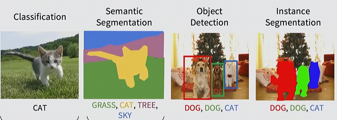
Common foundational computer-vision tasks include image classification, object detection, semantic segmentation, and instance segmentation.
In early July, my colleague Fufu from the platform team proposed an image-recognition-plus-raycast approach: use a small model to identify the Actors in a scene, then raycast to retrieve the corresponding Actor. In other words, object recognition followed by instance selection. This inserts a small visual-analysis model between the application and the LLM, letting the LLM actively acquire and segment the contents of the image.
By the way, placing an intermediate layer between a large model and an application is a wonderful agent-design trick. GSDL, which appears later, follows the same logic.
That proposal inspired me.
But it returns us to the same problem: if the model itself distinguishes objects directly from the image, it will sometimes fail, and the resulting analysis is unstable.
So why not reverse the direction? Let the engine report which Actor owns every pixel and output a mask table to the LLM, compensating for the model’s inability to separate every component of an image reliably.
That is my 2D asset-mask method. When the LLM asks for an image from a position, the editor responds. Optionally, instead of returning only the image, it also reports everything in the frame, compresses that visual information into text, and labels what every part of the image represents. The method slashes token cost while providing extremely stable, high-recall instance segmentation.
4.2 Establishing Visual Ownership
The editor already maintains a Hit Proxy rendering and readback mechanism so users can click objects. Its buffer corresponds to the viewport: every hittable pixel maps to a Hit Proxy, which can then be resolved back to an Actor, Component, or another editor object. We can reuse this mechanism and expose pixel ownership to the LLM. Compared with running a separate vision segmentation model, acquiring and parsing this data is cheap.


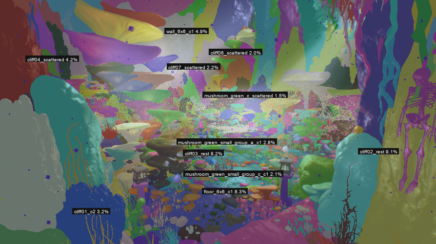
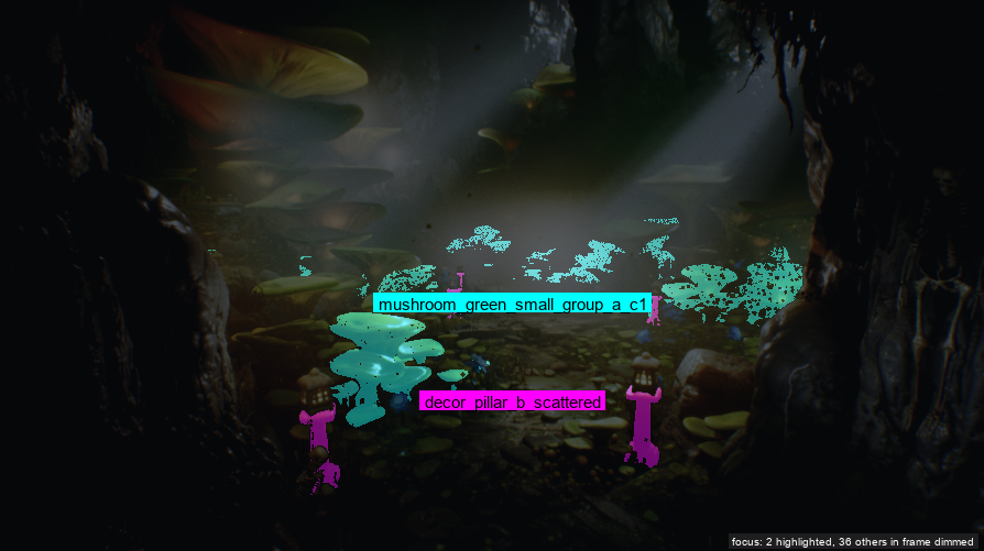
Once we know every Actor in the image, do we understand the image’s semantics?
Yes. Absolutely.
By a fortunate coincidence, I had just finished an asset-understanding tool—the previous installment in this series.


While building asset understanding, I generated a description for every asset—the left image above—and artists continue editing and improving those descriptions.
The mask statistics on the right reveal, among other things:
- how much of the image each asset occupies, how it is distributed, and how far away it is;
- which source asset it comes from, so it can link back to asset semantics;
- what the instance is called in the scene and which scene parameters it has.
4.3 Edge Cases and Local Vision-Model Support
Careful readers may have noticed that three kinds of “special asset” reported by Hit Proxy need dedicated channels. I handle each separately:
- Procedural foliage — split it apart and map each foliage Actor back to the semantics of its source asset.
- Terrain — Hit Proxy reports an entire Landscape Proxy: one name covering a huge swath of pixels. Artists, however, paint multiple user layers into the weightmap—grass, sand, snow, water, and so on. The integration layer therefore follows a dedicated route: world coordinate → proxy-local UV, calculated from proxy scale → weightmap texture sample →
ULandscapeLayerInfoObject::GetLayerName(). No visual inference is involved anywhere in the chain, which makes it highly stable. - Built-in engine objects such as sky and atmosphere — there are few of them, so I provide handwritten semantics rather than depending on Hit Proxy.
Now we give the VLM the descriptions + image + mask information, organized at several LoD levels, and ask it to generate a description of the frame. Yes, this is a model describing a description—recursion achieved. These LoD levels can be exposed as interface parameters for different levels of detail.
Here, LoD means the granularity of information shown to the model, not mesh geometric detail, although the numbering direction remains consistent.
We can go further by deploying a small vision-language model locally behind the MCP layer. For example, Qwen2.5-VL-7B int4 averages 5.95 GB of VRAM and peaks at 6.65 GB, small enough to run on most artists’ workstations. Deploying Qwen3.8 27B on the studio LAN is not especially difficult either.
Interpreting images and their attached information is a classic perception task and does not require a long chain of reasoning—the sweet spot for a small model. Modern VLMs are pre-trained on large image or image-text corpora and already possess basic visual-semantic ability. This local sidecar lets a cheap, effective, non-multimodal model such as DeepSeek V4 Flash 0731 use our visual-understanding layer as well.
Roughly speaking, a small model is sufficient on one side of the following boundary and begins to struggle on the other:
| Dimension | 🟢 A small model is enough | 🔴 A small model begins to struggle |
|---|---|---|
| Spatial | “There is a treasure chest / mushroom / rock / distant silhouette in the image” | “The exact distance between the chest and the nearest mushroom; back-projecting a precise 3D coordinate” |
| Visual | “Warm palette, cave atmosphere, low-poly style” | “A 0.7 silhouette deviation from the concept art; which subject damages the composition” |
| Semantic | “What is present”—perception | “Why was it placed this way, and how should it change?”—reasoning + decision-making |
The exact deployment choice naturally depends on the environment.
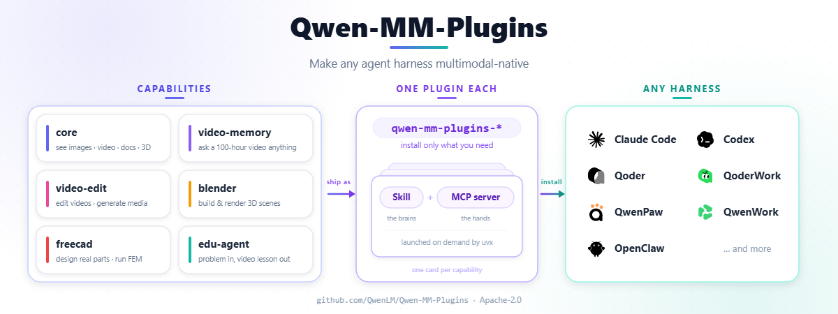
Update, August 10: Alibaba recently released Qwen-MM-Plugins, which is very close to my idea. It moves visual understanding into the harness layer and uses multi-resolution processing and frame sampling to understand images and video, essentially completing the sidecar capability I describe here. I will upgrade my approach accordingly.
With this framework, everything in an image can be assigned semantic ownership. Auxiliary objects that Hit Proxy never hits—post-process volumes, lights, and the like—leave no trace in an image mask, so we need another probing dimension.
Enter GSDL.
5. GSDL: The General Scene Description Language
Never heard of it?
Of course not. I made it up. 🐶
5.1 How Do We Understand Space?
The 2D mask method only fills half the gap. It tells the model what is in the image—visual information plus content semantics—but the spatial-relations row in the 3 × 3 matrix remains unsolved.
The editor was built for people. A person can glance at a viewport and immediately feel whether an area is dense or sparse, whether objects are scattered or huddled together. The editor cannot answer those questions directly.
The data we need is not hiding in a single engine field, waiting to be retrieved. It must be measured, aggregated, and inferred from Actors, coordinates, bounding boxes, collision, terrain, rays, and rendering results. The engine does not expose those conclusions as ready-made APIs. A person acquires them intuitively by walking through a scene; an LLM does not.
That is what GSDL does. Through measurement, it cooks and compresses low-level engine state into scene facts that an AI can query, compare, and verify: “there is a mountain at A,” “there is a depression at B,” and so on.
GSDL is also built on MCP, but it does not expose raw engine interfaces directly. A layer of GSDL query functions sits in between, and those functions are the language’s most important rules and conventions. Every query first performs its measurements inside the scene, then converts the result into standardized language for the LLM. In that sense, it can be viewed as an OpenUSD-like textual description language.
But “description language” only names the final output. More precisely, GSDL is a complete methodology for observing, measuring, and describing a scene for AI. One end connects to geometric and rendering facts in the engine; the other connects to asset semantics. Between them, it organizes what exists, how it is distributed, and how the pieces relate into structured language at multiple LoD levels for the LLM.
This diagram shows one complete query loop. MCP is only a thin wrapper: it does not do the work itself; it forwards calls into the engine.
① The model issues an MCP call—
describe_region,find_opening,compare, and so on—which arrives at ②, the MCP query interface: the GSDL query layer described above.② A file bridge carries the request into UE, where scene probes perform the actual measurements and produce raw, uncompressed facts.
③ The spatial kernel clusters those facts and infers relationships. The GSDL encoder then compresses them according to LoD and a character budget. Only then does the model receive the result.
After reading the result, the model reasons about what to measure next and returns to ① with a new question. The query keeps circling through this loop.
In short, GSDL has two main jobs:
- understand spatial information by organizing discrete objects into density, structure, relations, visibility, and semantic ownership;
- compress acquired information into concise but rigorously structured semantic statements.
Let us examine them separately.
5.2 How Is Space Measured?
I will visualize one interface so its implementation is easier to understand.
The interface is called find_opening. It tests whether a cavity contains openings. In a cave, for example, it can measure how many entrances exist; in a room, it can determine whether a window is open.
UE is an excellent simulation tool. There is a surprising amount of “measurement” you can do inside it.
The engine already exposes raycasting—LineTraceSingleByChannel in UE—as a native physics query. Walls, rocks, and doorframes are positive space. An opening is the negative space enclosed by them.
So find_opening does not search for Actors whose names contain Door or Archway. It works backward through collision queries: rays that hit geometry trace the walls of a cavity, while groups of rays that escape continuously into the distance indicate an opening. The system then returns to either side of that opening to measure the real frame.
The implementation can be divided into five steps:
- Find interior points. Lay down candidate samples inside the cavity and keep those that are genuinely enclosed.
- Choose observation stations. Select several spatially separated interior points as viewpoints.
- Cast rays. Fire rays around each station and find directions that escape into the distance.
- Fuse and classify. Combine observations from all stations and distinguish entrances, high windows, and internal passages.
- Measure exact dimensions. Return to the edges of each opening and measure its real width and height.
The low-level C++ Probe retrieves terrain, instances, collision hits, and ray results from the live Editor. A Python spatial kernel handles candidate sampling, station selection, sector fusion, classification, and precise-measurement scheduling. The LLM no longer receives more than ten thousand raw rays. It receives a compact set of scene facts with type, position, direction, width, height, source station, and evidence grade. It can quote the measurements directly or revisit the supplied camera positions for screenshot verification.
That is how we complete the spatial side of scene understanding.
5.3 How Is Language Compressed?
After the five measurement stages above, we are holding more than ten thousand rays, hundreds of sample points, and over three thousand instances. We cannot hand all that directly to the model—the context window would explode. This is why the earlier Canvas diagram includes a Python data-reduction layer between the raw probes and the LLM.
Compression here does not mean shortening sentences. It is a set of language-design principles:
- Description is not a data dump. The tool cooks raw instance data into statements: “this region contains 3,242 instances across 200 asset types, organized into 12 clusters; the largest cluster lies to the southeast…” If the text exceeds its budget, it automatically falls back to a coarser LoD. The underlying detail remains available at finer levels.
- Disclose progressively; summarize first. Descriptions have four levels, LoD0 through LoD3. LoD3 is a one-sentence summary. LoD2 is an asset inventory with statistics. LoD1 expands clusters and spatial relations. LoD0 preserves per-instance detail. The result is also divided into themed channels. By default, the model receives only LoD3: spend a few tokens deciding whether the region deserves attention, then drill down only when necessary—exactly how a person explores a scene, scanning from afar before walking closer.
- Aggregation is reversible. Compressed detail is not destroyed. LoD1 shows clusters; if the model wants LoD0 for one cluster,
expanddrills into only that cluster instead of describing the whole region again. - Truncation must confess. Every compressed or sampled result says so:
truncated (~30% sampled),(3 of 148), or an approximate value prefixed with~. Every number tells the model whether it came from the full population or a sample.
This is what I meant earlier by “compressing acquired information into rigorously structured semantic expression”: we compress tokens while progressive disclosure preserves access to the information.
Here is the token cost of four output levels for the same describe_region query:
| Output form | What the model receives | Characters | ≈ tokens |
|---|---|---|---|
| Raw JSON data dump | One coordinate array per instance | 461,193 | ~115,000 |
| LoD3 summary | One sentence | 244 | 61 |
| LoD2 inventory | Asset inventory + density statistics | 840 | 210 |
| LoD1 relations | Clusters + spatial relations + statistics | 2,616 | 654 |
| LoD0 detail, one expanded cluster | One category only: a 20-instance scattered-rock cluster | 1,687 | 421 |
| LoD0 detail, entire region | One or two lines per instance, about 23 tokens each. The system never normally requests an entire region this way. A forced full dump can even exceed raw JSON because GSDL carries many annotations. | 921,223 | ~230,000 |
Here is the complete LoD3 result:
1 | @gsdl v0.1 |
Line by line:
@gsdl v0.1— the version declaration.@project: ScatterTest— the map or project being observed.@asset_classes: [Foliage, StaticMesh]— the broad asset classes present in the region.@enrichment: []— the semantic-enrichment slot, connected to the asset-semantic encoding from Form 1. It is empty in this example.@frame: m— the unit contract. Every following length is in meters and every angle is a compass angle, so the model never has to guess whether92.05means centimeters or meters.region(id=R7, bbox=[0.0..200.0, 0.0..200.0, 0.0..18.0]m)— the region envelope. Every statement inside the braces applies to exactly this bounding box and not an inch beyond it.# -- summary (LoD3) --— a channel heading that identifies the theme of the following block.R7 summary ...— the only body sentence and the only sentence form in the entire output: a triple. The subject is R7, the predicate issummary, and the object is a semicolon-separated compressed statement terminated by a period. Predicates come from a fixed vocabulary—located_at,bound,near,density, and so on—rather than free-form prose.
Inside that predicate:
anchor=watch_tower names the landmark. The anchor is selected by salience—visual area × rarity. Among ten thousand six-meter pine trees, only the eighteen-meter watchtower deserves the title. Every later cluster relation hangs from it: pine_c2 of watch_tower or pine_c2 offset (dir=NE, d=43.2m) uses the tower as an origin. 10021 instances/3 classes reports scale, density=0.25/m² reports spacing, and orientation=scattered is a binned orientation-entropy result: ordered placement or disorder.
People give directions in the same order: first a landmark—“near Black Well”—then a relative comparison—“darker than the cave at Flower-Fruit Mountain.” The anchor turns that human habit into grammar.
Two other grammatical elements are not visible in this sample.
The first is precision marking:
- measured values have no prefix:
pine_c1.1 pose [92.05, 12.65, 0.0]m; every number was measured; - estimated values use
~:watch_tower salience ~1.00; salience is a calculated estimate; - classifications use
#:size_dist {M:20, L:10001}#; bins are rule-based judgments rather than direct measurements.
The second is reference resolution. Similar objects are combined into clusters and the long tail is merged into a diffuse field. No matter how many instances exist, the language usually collapses them into only a dozen or so names. If you have a box of pencils, you do not need to say “pencil A, pencil B, pencil C…” Clustering is another form of referential compression.
Anchor, scale, density, and orientation all fit into those 61 tokens. The model can drill into whichever part it cares about.
LoD0 gives each instance one or two lines:
1 | pine_c1.1 pose [92.05, 12.65, 0.0]m @ yaw=99.7°. |
The model calls the appropriate interface itself to retrieve the detail it needs.
Do you remember the 3 × 3 understanding/expression matrix from Chapter 2? I proposed three expression strategies: reference, comparison, and metaphor. Now we can evaluate them.
Reference is exactly what anchors and clusters provide. pine_c2 and “the group northeast of the watchtower” refer to the same thing. offset (dir=NE, d=43.2m) is the formal version of “near Black Well.”
Comparison is quantized in GSDL. The system can provide precise numbers and comparative bands. But bands require quantization and judgment, and judgment introduces instability. That is why comparison received an orange, hard rating in the matrix.
The third strategy, metaphor—“this cave looks like the White Bone Demon’s lair”—is genuinely difficult. It depends partly on the LLM’s own understanding and partly on Vector Atlas, introduced later, which needs artists to teach and annotate scene semantics.
5.4 Self-Evolving Interfaces
The interface above is only one example. Around July 20, 2026, GSDL’s measurable spatial capabilities looked roughly like this:
| Capability | Representative interfaces | Core implementation | Questions it can answer |
|---|---|---|---|
| Topology | compare(on="spatial"), query |
World-AABB reasoning using RCC-8; scale-adaptive tolerances; DC / EC / PO / TPP relation codes | Are they disconnected, touching, overlapping, or contained? |
| Direction | compare(on="spatial"), describe_region |
Eight compass directions; facing / parallel / opposed / oblique orientation | Which side is A on? Are they facing or back-to-back? |
| Distance | compare(on="spatial"), query |
AABB surface gap, center distance, vertical offset; footprint-scaled near levels |
How far apart? Which is higher? Does this count as “next to”? |
| Support | describe_region, relation_trace, compare |
Vertical contact + footprint overlap as support evidence; sparse support graph | What supports what? “The cup is on the table” becomes a measurement. |
| Passage and occlusion | find_opening, skyline, query_view, rays / los_ring |
Multi-station rays, escape-direction clustering, frame remeasurement; viewpoint-relative occlusion jointly verified by rays and masks | How many exits does the cave have? What blocks the view? |
Those capabilities correspond directly to the spatial relations discussed above. GSDL also includes supporting spatial capabilities:
| Capability | Representative interfaces | Core implementation | Questions it can answer |
|---|---|---|---|
| Survey | scan_density, describe_region |
Enumerate Actors / Instances / Landscape; grid aggregation; snapshots, clusters, layered summaries | What is here? Where is it concentrated? Scattered or clustered? |
| Localization | search_subjects, find_by_class, actor_meta, semantic_search |
Name and Chinese-alias indexes, class queries, asset-metadata joins, cross-checking retrieval results against instances | What is the “treasure chest” called? Where is it? Which asset does it use? |
Before discussing spatial relations, the LLM must first know what exists and which instance a phrase refers to. Only then does it call the deeper reasoning interfaces.
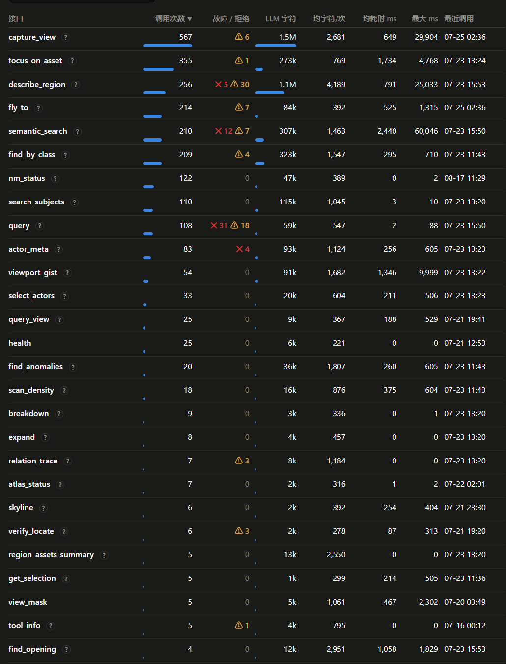
GSDL exposes a growing collection of question-oriented measurement capabilities. The list was not designed all at once; each evaluation round pushed it in a new direction. What you see above is only one snapshot in time. At present there are roughly 35 interfaces, about 20 of which are stable.
I first tried iterating on them in the conventional way. The result was negligible, mainly because iteration was too slow and my own judgment too subjective. I later switched to evaluation-driven development with /Loop: establish a bank of scene questions, have an LLM judge each round from its execution traces and answers, then let those results drive the next interface change. The improvement was dramatic.
My /Loop process has two stages.
For the first stage, I wrote 36 test questions by hand. The earliest bank contained only 11 questions; I later expanded it to 36, manually phrasing every question and annotating every answer. It nearly killed me.
The questions cover more than a dozen categories, including:
- Description and understanding: what is visible in the current viewport, how a district is planned, and how its functions are divided.
- Spatial relations: how far A is from B, in which direction, which is higher, and which blocks the other.
- Anomaly detection: floating objects, intersections, and obviously misplaced assets.
- Passage structure: how many openings a cave has and how wide they are.
- Composite decomposition: which six of fourteen archway assets form one complete gate, or which components make up a fortified enclosure.
- Honest denial: if the scene contains no cars and no neon, can the model say “none” with evidence instead of hallucinating one?
Every question is written in natural language and deliberately avoids naming any tool.
I run the /Loop with two agents. One runs the evaluation: it opens N subagents with clean contexts and asks each to call MCP; a Fable 5 lead agent only schedules work, writes the summary, and produces requirements. The other changes the code: Opus or GLM 5.2 optimizes the interface logic from those requirements.
The MCP-testing subagents use local Qwen3.6 27B and MiniMax M3. SOTA models do achieve higher completion rates, but production-scale MCP usage can become frighteningly expensive. These tools are meant for production, not leaderboards, so they must be adapted to the models that will actually be deployed.
I focus on three hard groups of metrics:
- Delivery: completion rate, accuracy, and honesty.
- Cost: actual token usage, interface call count, and the interface-schema tax.
- Speed: time per question, average latency in milliseconds, maximum latency, and watchdog timeout count. I sometimes also track health and discoverability.
Large and small models differ sharply in some respects, particularly tool use. Small models often forget which interfaces exist. I eventually built a routing layer that the model can call before querying the scene, so it can confirm which tool is appropriate. This trades more routing calls for a higher completion rate:

Here is how the three hard metrics changed, using ten questions under the same protocol on July 21–22:

Within a few days, tokens fell by 54%, calls fell by 64%, and the system reached a perfect score and held it.
I later expanded the question bank. After more than ten additional rounds, the metrics flattened out. Pushing further no longer made much sense; overfitting began to appear.
Time for a stronger dose.
That brought me to the second stage of /Loop development:
I built a passive-update system. When users call MCP tools during their normal work, a Hook records the exact question and the conversation in a background database. Users are also occasionally asked to rate how completely the LLM finished the task.
A scheduled agent turns those interaction records into a capability-requirements table whenever it detects a weak area. At night, after I leave work, an executor agent implements the capability. Another lead agent then launches many subagents to test the MCP changes, summarizes their reports and recommendations, and feeds them back to the executor. The executor iterates again. The loop continues until the new interface stabilizes.
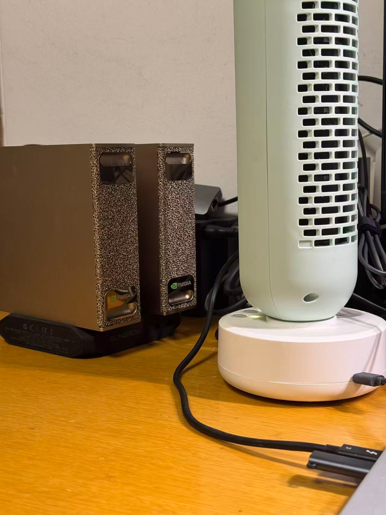
To make this loop work, I even bought two DGX Sparks to run DeepSeek V4 Flash locally. They are chewing grass as I write this—an otherwise pointless display of armament. I hope my Leader sees this paragraph and gives me a raise. ლ(╹◡╹ლ)
The /Loop is still not as complete as I want. I am continuously tuning it, and it contains far more concerns than the sketch suggests: user authorization, data redaction, sandboxing, audit, rollback, and so on. That is another subject I want to cover next time: a self-evolving agent system driven by real user data.
5.5 A GSDL Call in Practice
Here is one real GSDL invocation from a test I ran on July 23, 2026:
“How many passable openings does this cave have, and how wide is each one?”
It neatly illustrates the difference between “reading Actors” and “understanding space.”
Without GSDL—for example, with a conventional UE MCP approach—the LLM searches for assets whose names contain Archway and treats components such as SM_WallArchway_12x3 and SM_WallArchway_3x6 as openings. In my test, those Archway Actors were the walls surrounding the openings, not the openings themselves, so the model misclassified them.
With GSDL:
1 | → nm_status ← confirm tool status |
Before the find_opening route existed, the model used 47 tool calls and consumed 64,820 returned characters, yet still mistook wall components containing Archway for entrances. After routing was added, it needed only five calls and 15,540 characters to complete both measurement and visual verification.


The model then flew to each candidate opening and captured a verification image. The mask contained 494 pixels belonging to BP_Sky_Sphere, showing that the line of sight passed through the opening into the outside background. That is only visual supporting evidence for the opening’s existence. Whether it is passable and how wide it is still come from collision rays near the ground and precise frame measurements.
In the end, the system classified ten candidate structures into ground-level passable openings or passages, elevated windows, and skylights, then reported the positions and measured widths of the ground openings. It even found an opening I had never noticed. The important point is not “how many Actors named Archway did it find?” It is that the system can distinguish a cave wall, an internal passage, an exterior entrance, and an elevated opening that cannot be traversed directly.
5.6 Open-Sourcing the Project
Thank you for making it this far.
Once this busy period is over and the company-specific material has been separated, I will open-source GSDL on GitHub. I would be delighted if people tried it and sent suggestions; one person’s energy is simply too limited.
The repository placeholder is already here: OpenGSDL. I expect to upload the code in early September. It will contain both the mask method and GSDL, packaged as a multi-version UE MCP plugin that you can extend or use alongside Epic’s official MCP.
6. Vector Atlas: Semantic Encoding for the Entire Map
I built Vector Atlas because every live model query against a map is painfully slow. It has to load a scene, acquire masks, capture screenshots, and so on. In our project, one such operation takes at least 60 seconds. Searching across an entire world multiplies that latency dramatically. Could the process be made much faster?
I also need far more semantic information about the scene. Artists must annotate much of it; I could never label an entire large map alone. Scene semantics—“this is a particular NPC’s house,” for example—also change as production evolves and therefore cannot be hard-coded. I need a dynamic, editable service for collecting scene semantics.
That is why I built Vector Atlas, a semantic encoding of the whole map.
It combines the 2D mask method and GSDL.
Encode every map offline into a semantically searchable table of viewpoints. People can search the entire map by meaning, add viewpoints manually, and edit their semantics. The same structure also becomes cross-session long-term memory for AI: an agent can add a viewpoint, preserve it as a memory, and retrieve it later.
The promise from the beginning—to “memorize” every place and query it in milliseconds—is fulfilled here. It is an engineered trade: storage for performance.
This article is already far too long, and Vector Atlas is itself a very complicated project. How should search be optimized? How should viewpoints be captured? How should it be deployed? How can the system infer an angle it never photographed? Each question deserves serious thought.
So Vector Atlas, together with the real-user-data self-evolving agent system introduced above, will be the subject of the next article. By then, the system should also be more complete.
For now, here is a short tool demo.
7. The Version for Carbon-Based Lifeforms
8. The Version for Silicon-Based Lifeforms—and a Comparison with Epic’s Approach
I prepared 11 questions and had each model use either Epic’s official MCP or my MCP, NeuroMap build 08-14. Every question started from a clean context, and I repeated the evaluation with three models.
| Metric | DSV4flash + local Qwen3.5-9B-4bit Epic |
DSV4flash + local Qwen3.5-9B-4bit NeuroMap |
Qwen3.8 27B Epic |
Qwen3.8 27B NeuroMap |
GPT-5.6 Luna Epic |
GPT-5.6 Luna NeuroMap |
|---|---|---|---|---|---|---|
| Harness | Claude Code | Claude Code | Claude Code | Claude Code | Codex | Codex |
| Completion rate | 100% (11/11) | 100% (11/11) | 72.7% (8/11) | 90.9% (10/11) | 100% (11/11) | 100% (11/11) |
| Accuracy | 77.3% | 77.3% | 59.1% | 86.4% | 90.9% | 90.9% |
| Honesty | 95.5% | 90.9% | 68.2% | 72.7% | 86.4% | 90.9% |
| Total time, official primary runs | 468m 7.0s | 64m 52.2s | 611m 8.9s | 291m 21.8s | 141m 35.5s | 40m 3.6s |
| Mean time across all 11 questions | 42m 33.4s | 5m 53.8s | 55m 33.5s | 26m 29.3s | 12m 52.3s | 3m 38.5s |
| Maximum time for one question | 197m 4.3s | 20m 15.0s | 220m 3.8s | 84m 50.3s | 52m 1.6s | 18m 6.3s |
| Total MCP calls | 514 | 261 | 318 | 221 | 7,919 | 313 |
| Input / output | 20,179,996 / 261,572 | 6,158,052 / 119,825 | 10,173,709 / 234,831 | 8,438,133 / 150,085 | 47,692,261 / 207,474 | 21,170,665 / 94,384 |
| Fixed first-turn overhead | 700 tokens | 12,326 tokens | 569 tokens | 14,761 tokens | ~350 tokens | ~12,900 tokens |
Overall, NeuroMap matched or exceeded delivery quality while sharply reducing tool calls and runtime. In the Luna evaluation, Epic’s MCP made 7,919 calls; NeuroMap made only 313, about one twenty-fifth as many, and took only 28% of the total time.
Epic’s MCP exposes general-purpose, atomic editor operations. The model must route repeatedly and inspect objects one by one—almost a traversal of every Actor in the scene. As scene complexity grows, one question can fragment into hundreds or thousands of calls, and round-trip overhead expands rapidly. NeuroMap aggregates region description, anomaly detection, opening analysis, and other spatial computation on the UE side, then compresses the result with GSDL. Across all three models, that produced fewer calls, shorter long tails, and higher delivery rates.
The most striking accuracy result came from Qwen: my MCP raised accuracy from 59.1% to 86.4%. Aggregated, problem-oriented tools are not merely cheaper; they also reduce the burden on a weaker model that would otherwise have to traverse Actors, choose tools, and infer spatial relations by itself.
NeuroMap still has a relatively high schema overhead, and its tool set continues to be consolidated. There is more optimization ahead.
The following is one real workflow. The AI receives only a vague description—“a table with a Go board on top”—then locates it in a large scene, adjusts the camera, and saves a screenshot.


9. Afterword
Have you noticed something? NeuroBrowser—the plugin from Form 1—and NeuroMap—the plugin from this installment—both inject AI capabilities into the engine editor. Their initials are NB and NM; internally, the Chinese pronunciation gave them the nicknames “Your Dad” and “Your Mom.” Together, they feel a little like rebuilding the editor around AI capabilities.
Perhaps this is what the next generation of game editors should look like.
What do you think?